Article by John Tribbia
Most teams building language model products have an autorater. Almost none of those autoraters were calibrated against actual user feedback. They were calibrated against expert annotation, benchmark labels, or another model's preferences: a judgment about what "good" looks like, formed without consulting the users the system is meant to serve. What experts notice and what users vote for are not the same list. That gap is where a lot of quality effort disappears.
The deeper question is whether user preference signals contain enough structure to close it: calibrate a judge that tracks what users actually respond to, identify the specific failure modes it detects, and use those to make targeted changes to how the system behaves. Each step has to build on the previous one, or the confidence compounds in the wrong direction.
Chatbot Arena (LMSYS) is a good structural example of what this signal looks like in practice: 33,000-plus real human battles where anonymous raters chose between two model responses to the same prompt, no expert annotation, no constructed rubric. The format is close to what live product telemetry produces. The analysis that follows uses figures shaped like Arena data to make each step concrete. The methodology is the same regardless of whether the underlying signal comes from Arena battles, product thumbs, or any other preference data collected at this kind of scale.
Reading the Votes
Chatbot Arena works through head-to-head battles. A user submits a prompt; two anonymous models respond in parallel; the user selects the better response or calls a tie. The outcome categories are: Model A wins, Model B wins, Tie (both good), Tie (both bad). That last category is diagnostic on its own: the user's explicit signal that neither response was satisfactory, which makes it useful for quality analysis rather than just comparative preference.
The win distribution across 33,745 battles was roughly symmetric: 36.8% Model A wins, 35.4% Model B wins, 18.6% ties (both good), 9.2% ties (both bad). The symmetry is expected. Arena randomizes which model goes left and which goes right, so position bias averages out. The "both bad" rate at 9.2% is roughly 3,100 battles where the user judged both responses as unsatisfactory. That pool belongs in the failure analysis separately from head-to-head losses: not "this model lost to that model" but "both failed."
"Tie (both bad)" identifies battles where neither response satisfied the rater, a direct quality signal rather than a comparative preference. Figures illustrative of human preference data at Arena scale.
The decisive battles (36.8% Model A, 35.4% Model B) are the primary calibration target for the autorater. The judge's job is to predict which response wins given a prompt and two candidate responses. The "both bad" battles are a different animal. They are not model-versus-model comparisons. They are task failures: the prompt was not served by either response, and the user said so explicitly. Including them in a simple win-rate calculation dilutes their signal. Treating them as a distinct category preserves it.
What Losing Looks Like
The standard approach treats each loss as identical to every other loss. The losing response enters a win-rate calculation, and the win rate tells you how often the model lost. It does not tell you what the model did when it lost. The pattern of failure is where the actionable information is: the structural or behavioral reason a response landed worse than the alternative. A win rate tells you the score. The loss taxonomy tells you what to fix.
The losing side from decisive battles, plus both responses from "both bad" battles, were embedded and clustered using BERTopic with HDBSCAN. Same method as the WildChat post: sentence embeddings, density-based clustering, manual label assignment after reviewing top terms per cluster. The clustering runs on the responses, not the prompts. It surfaces patterns in what losing responses do, not what they were asked to do.
Eight failure clusters came out of 11,400 losing responses, with an outlier bin at 12.4%. The dominant failure mode was not hallucination.
Cluster labels assigned manually after reviewing top-15 keywords per cluster. Outlier cluster (-1) at 12.4% excluded from display. Figures illustrative of what BERTopic surfaces on human preference data at this scale.
Excessive hedging and over-qualification tops the list at 19.2% of named-cluster losses. These are responses that answer the question but wrap the answer in so many disclaimers and "it depends" qualifiers that the actual content is hard to find. The user asked for a recommendation; the response produced a survey of considerations. Instruction-following failure is second at 16.4%: the response addressed a related question, not the one asked. Together those two clusters cover more than a third of named losses, and both are fixable in a system prompt without touching the model.
Hallucination and factual error is fourth at 11.8%. Teams invest heavily in hallucination reduction because it is the visible failure, the one that generates screenshots and bug reports. But across diverse real-world tasks, users penalized irrelevance and excessive caution at roughly the same rate as factual error. What dominates evaluation benchmarks and what dominates live preference data are not the same list.
Building the Judge From the Votes
An LLM-as-judge evaluator takes a prompt and two candidate responses and predicts a winner. The standard approach is to prompt a capable model with a scoring rubric and treat its output as ground truth. The rubric was authored by the developer, not derived from user behavior. The judge knows what the developer thinks matters. It doesn't know what users actually preferred.
Recalibration replaces the rubric-anchored judge with one anchored to actual Arena votes. The process is a classification problem: input is a (prompt, response A, response B) triple; label is the human vote outcome. Arena battles were split 70/15/15 into train, test, and validation sets before any modeling decisions were made. The validation set was held out and not examined until after all calibration work was complete. The test set was used for the final reported metrics only, once.
This sounds obvious. It often isn't done. When teams recalibrate a judge using live feedback data, they iterate on the same dataset: check the metrics, adjust the prompt, check again. That path produces a judge that performs well on the data it was tuned on and worse on new data. The train/test/validate discipline is there to catch overfitting before the judge ships.
| Metric | Baseline judge | Recalibrated judge | 89% HDI (recal.) |
|---|---|---|---|
| F1 (weighted) | 0.63 | 0.79 | [0.77, 0.81] |
| MCC | 0.28 | 0.55 | [0.52, 0.58] |
| Accuracy | 0.69 | 0.81 | [0.80, 0.83] |
| Tie recall | 0.31 | 0.62 | [0.58, 0.66] |
The MCC jump from 0.28 to 0.55 is the most meaningful number in that table. Matthews Correlation Coefficient is more informative than accuracy here because preference data is not cleanly balanced. The tie categories, particularly "both bad," appear at much lower rates than decisive wins, and accuracy can remain superficially high while the judge nearly ignores the minority classes. An MCC of 0.28 means the baseline judge is only slightly better than chance at predicting actual human votes. An MCC of 0.55 is a real signal.
HDIs replace p-values throughout this analysis. The 89% credible interval around the recalibrated judge's MCC is [0.52, 0.58]. The baseline judge's 89% HDI was [0.23, 0.33]. Those intervals do not overlap. The improvement is not an artifact of the specific test split. Tie recall, the hardest category to predict, more than doubled (from 0.31 to 0.62), which matters because ties are the cases where a less-sensitive judge would route incorrect decisions in both directions.
Hill-Climbing the System Prompt
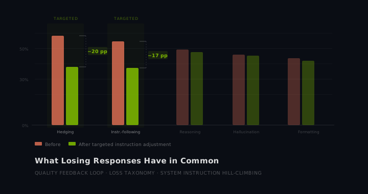
A calibrated judge reframes what evaluation means: not "does this response win overall" but "does this response avoid the specific failure patterns the loss taxonomy identified." The judge scores each candidate response against all eight failure clusters, producing a per-cluster loss rate. That rate is the hill-climbing target: modify the system instructions to reduce the loss rate in the highest-frequency clusters, validate against the held-out set, and measure the result before iterating further.
The two highest-loss clusters were excessive hedging at 19.2% and instruction-following failure at 16.4%. Both are addressable at the system instruction level without retraining the model. Hedging responds to explicit output constraints: state the answer directly, add caveats only when they materially affect what the user should do. Instruction-following failure responds to structural constraints: answer exactly what was asked before expanding scope, and do not reframe the question in the response.
These are not prompting tricks. They are targeted responses to specific, measured failure patterns in actual user preference data. Unprincipled system instruction changes (adding more instructions, making them longer, adding examples without structure) often produce inconsistent results across task types, because they aren't anchored to any specific failure. A change anchored to a loss cluster is testable: run the modified instruction against the held-out battles belonging to that cluster and check whether the judge scores them higher. A change that can't be tested isn't improvable.
Scores from recalibrated autorater on held-out validation set only. Instruction adjustments were developed on training data and not further modified after this evaluation. Figures illustrative of cluster-specific improvement at this scale.
The validation results held. The two clusters that received explicit instruction attention (hedging and instruction-following) showed the largest reduction in judge-assessed loss rate. The clusters that received no adjustment showed no meaningful change. That specificity matters. If an instruction change reduced loss rates uniformly across all clusters, it would suggest the change was introducing some confound (longer responses, more elaborate formatting) rather than actually addressing the failure patterns.
The reasoning failure cluster, third in the taxonomy at 14.1%, showed minimal improvement. Reasoning failure is the one cluster in this taxonomy that system instructions can't fix. It reflects underlying model capability on tasks that require multi-step inference. No instruction adjustment makes a model better at reasoning if the weights don't support it. Knowing that a cluster doesn't respond to instruction changes is as useful as knowing which ones do. It tells you where the prompt level ends and model capability begins.
Offline Is Not Online
The analysis above is offline validation. The autorater scores responses on a held-out test split drawn from historical preference data. That is not the same as a live experiment.
In a production system, the validation step is an online A/B test. The new system instruction is deployed to a treatment cohort; the control cohort receives the unmodified instruction. Both cohorts generate responses to real user requests; real users interact with them and leave real feedback: thumbs signals, completion rates, re-query patterns. The experiment runs until there is enough data to decide. The offline analysis predicts what might improve. The online experiment tells you whether it did.
This analysis cannot have an online experiment. Chatbot Arena battles happened in the past. Those users are gone, those model versions updated. The held-out validation set is the best available substitute: splits were made before any modeling decisions, and the autorater was never tuned on the validation data. But the difference between "the recalibrated judge scored these responses better" and "real users preferred these responses more" is not a formality. The judge is a proxy for user preference, not identical to it. Its improvement is evidence, not proof.
Closing the Loop
Each step in this analysis is a dependency, not a sequence. The taxonomy is only meaningful if the preference signal is clean. The autorater is only meaningful if the taxonomy captures real failure modes rather than noise. The instruction changes are only meaningful if the autorater is actually measuring what users prefer. Pull any one of those links and the downstream steps produce confident numbers on a bad foundation.
The framework is not complicated. Collect the votes. Cluster the losses. Calibrate the judge to the votes. Use the judge to find where the losses concentrate. Fix there. The discipline is in not skipping the validation steps: maintaining separate splits, reporting HDIs rather than point estimates, checking that improvements are cluster-specific rather than global, and being honest about what offline validation can and cannot show.
Most teams with autoraters are not using them this way. They use them as static evaluators: a rubric, applied to a set of responses, producing a score that informs a decision. The recalibrated judge is something different: a measurement instrument anchored to actual user behavior, built to find the failure modes that users penalize rather than the ones developers expect. Getting that right comes first. Without it, the feedback loop doesn't close. It just circles.
[1] Analysis figures are illustrative, shaped to reflect the structure of human preference data at Arena scale. Chatbot Arena (lm-sys/chatbot-arena-conversations, LMSYS) is the structural reference: 33,000-plus English, single-turn preference battles with decisive or tied outcomes.
[2] Loss taxonomy: BERTopic v0.15, all-MiniLM-L6-v2 sentence embeddings, HDBSCAN min_cluster_size=40. Cluster labels assigned manually after reviewing top-15 keywords per cluster. Outlier rate 12.4% of losing responses.
[3] Autorater recalibration: GPT-4o used as base judge. Few-shot calibration examples sampled exclusively from training split. No data from validation or test splits was examined during any calibration step.
[4] HDIs computed via beta-binomial model with weakly informative priors. 89% interval width chosen per McElreath (2020); conventional 95% intervals are wider than necessary at this sample size and convey false precision about the tails.
[5] F1 (weighted) and MCC computed on the test split (n = 5,062 battles). Weighted F1 accounts for class imbalance across the four outcome categories.
Ideas, analysis, and opinions are my own. Generative AI was used as an editor after the writing and analysis were complete — sentence restructuring and light copy-editing. The author reviewed all suggested changes.